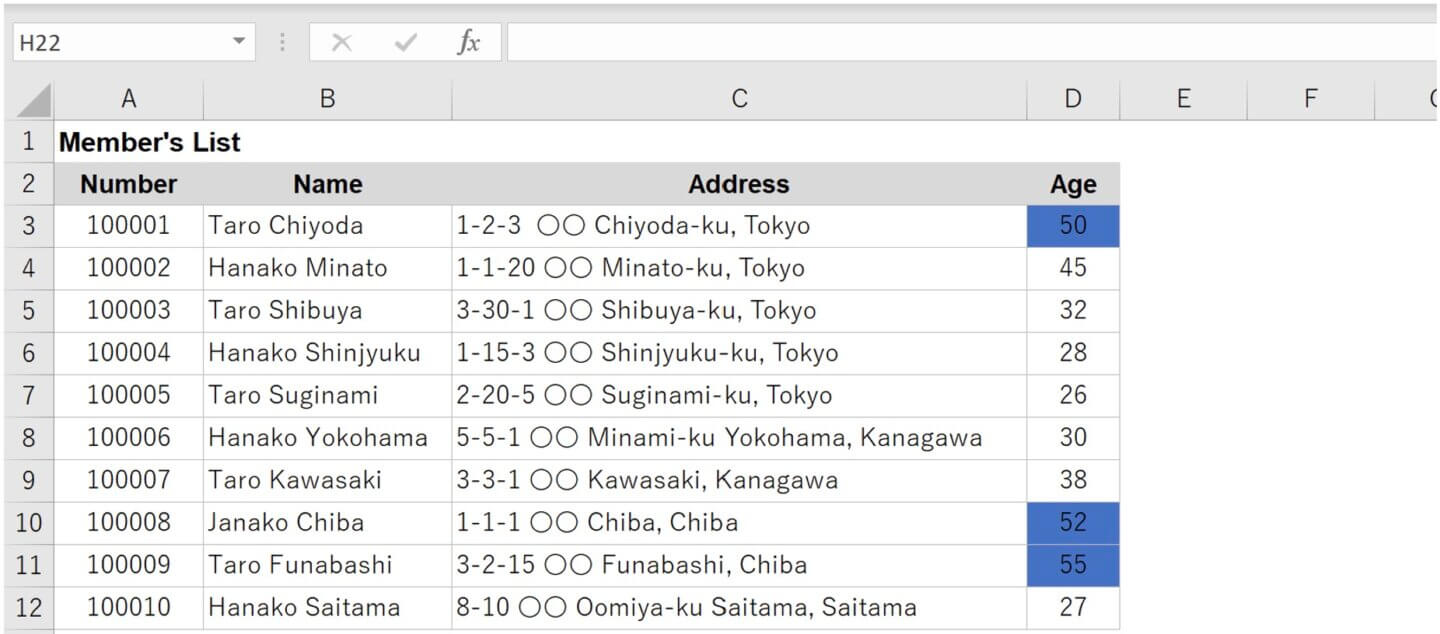
An Excel feature called Conditional Formatting allows you to highlight cells or rows that contain a specific string or match a condition with a color. For example, you can highlight the cells containing “Tokyo” in the address or highlight the rows for members over 50 years old in the following member’s list.
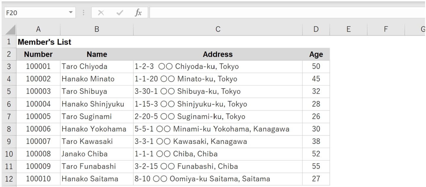
In this article, you will learn how to highlight the cells or rows for members over 50 years old.
Language: English Japanese
–
1. Highlight the cells that match a condition
Let’s highlight the cells in blue for members over 50 years old. When setting up conditional formatting, three things are required: Range, Condition, and Format.
| Range | Cell D3:D12 |
| Condition | Over 50 years old |
| Format | Fill in Blue |
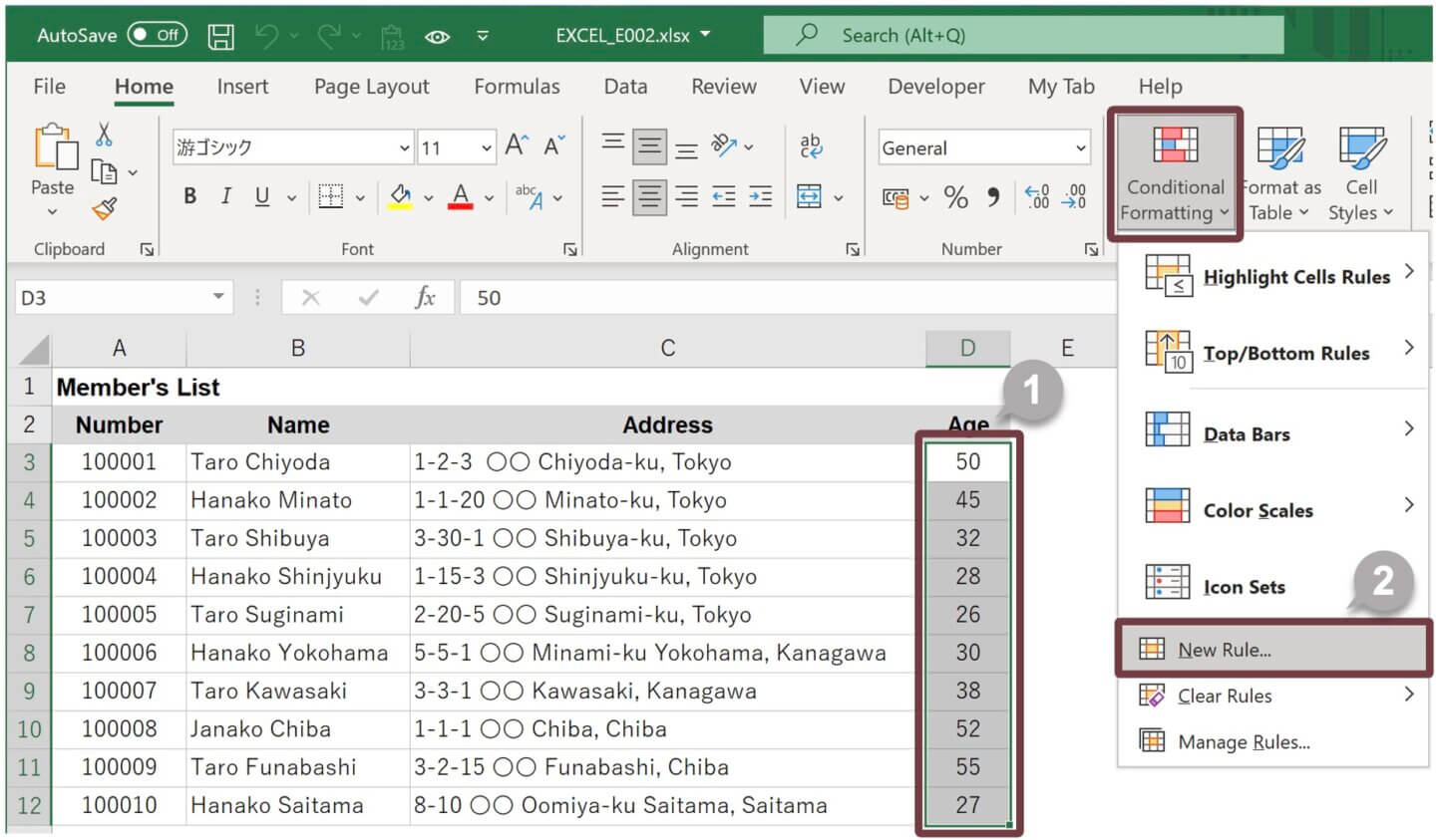
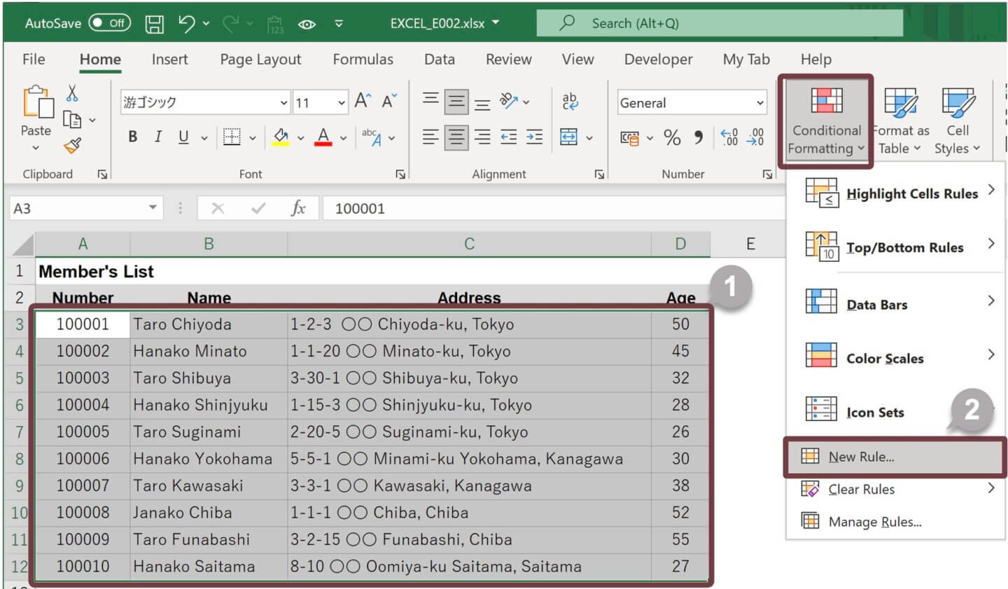
1 Select the range D3:D12 where you want to set the conditional format.
2 In the Styles group on the Home tab, click on Conditional Formatting and select New Rule from the list.
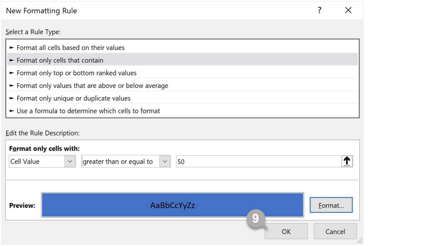
3 The New Formatting Rule dialog box will appear.
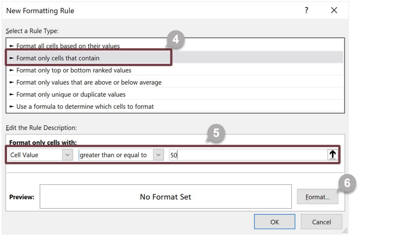
4 Select [ Format only cells that contain ] for a rule type.
5 Select [ Cell Value ] and [ greater than or equal to ] and type [ 50 ] for the rule description.
6 Click on the Format button.
7 The Format Cells dialog box will appear.
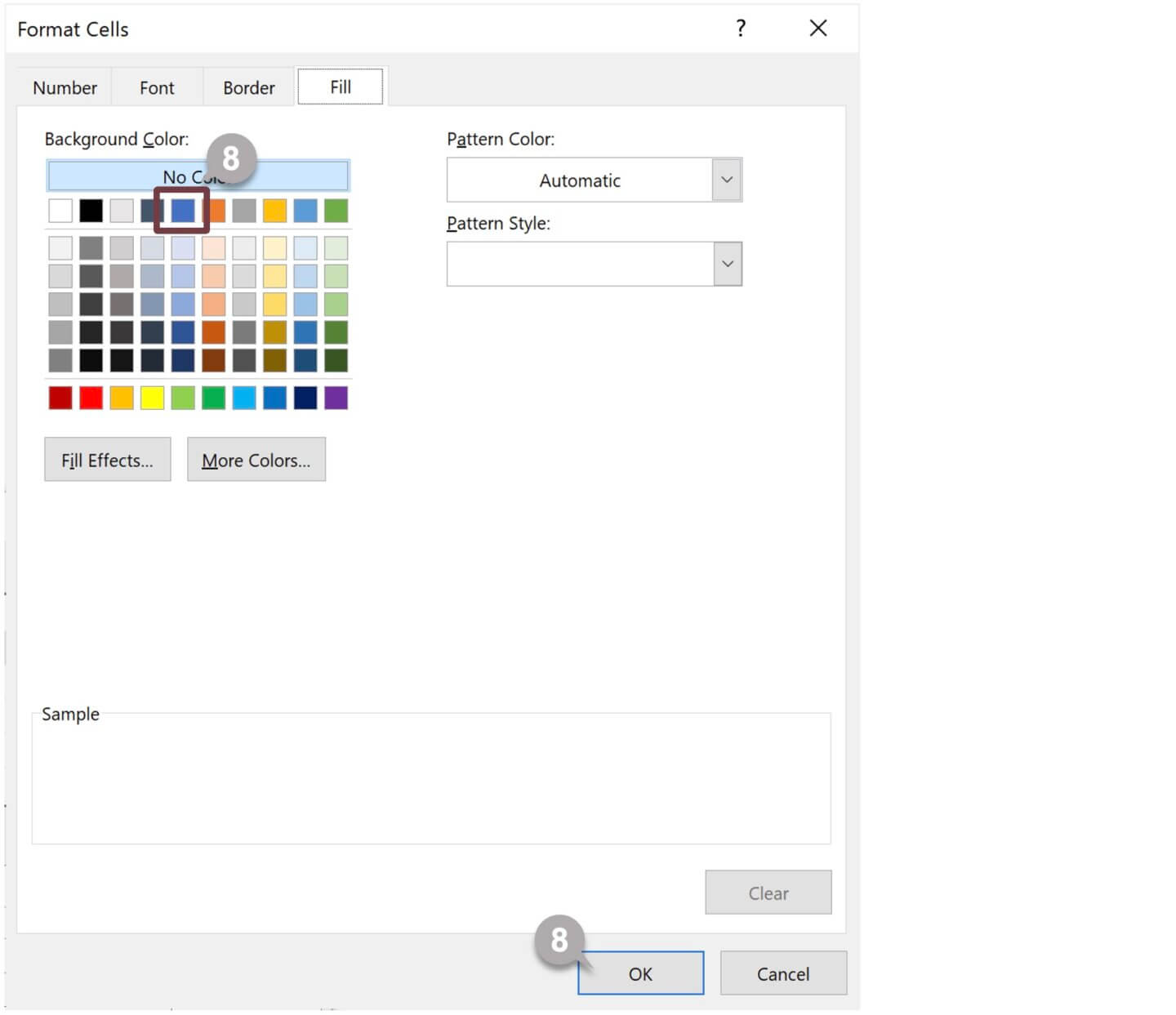
8 Click the Fill tab, select a blue color and click the OK button.
9 Click on the OK button.
10 The cells for members over 50 years old will be highlighted.
2. Highlight the rows that match a condition
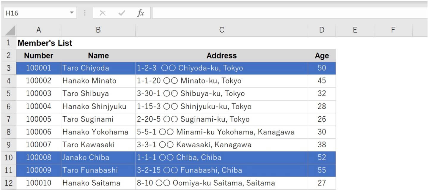
Let’s highlight the rows in blue and the text in white for members over 50 years old. The condition is to highlight the row if the value entered in column D is greater than or equal to 50.
First, let’s look at the first line of the list. Set up a rule such as [ =D3>=50 ] in cells A3, B3, C3, and D3. Setting conditional formatting for each cell is time-consuming, so set the range as [ A3:D3 ]. The conditional formatting rule is as below.
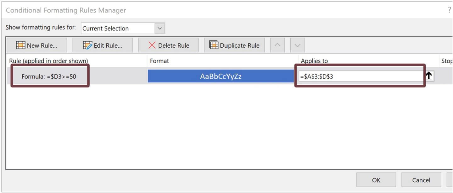
The point is the [ $D ] in the formula [ =$D3>=50 ]. Make column D an absolute reference, that is, fix column D. In the case of the formula [ =D3>=50 ], column D is not fixed, so the rule for cells B3 to D3 will be set as follows
| Applies to | Rule (Formula) |
|---|---|
| Cell B3 | E3>=50 |
| Cell C3 | F3>=50 |
| Cell D3 | G3>=50 |
In this case, if you type 50 in cell E3, cell B3 will be highlighted. Now let’s try to set conditional formatting for the entire list.
1 Select the range A3:D12 where you want to set the conditional format.
2 In the Styles group on the Home tab, click on Conditional Formatting and select New Rule from the list.
3 The New Formatting Rule dialog box will appear.
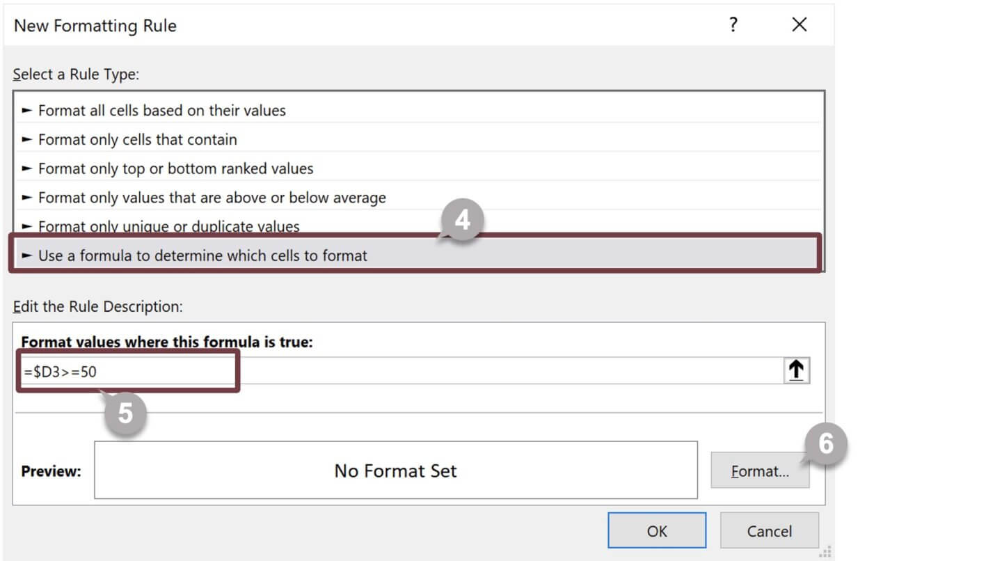
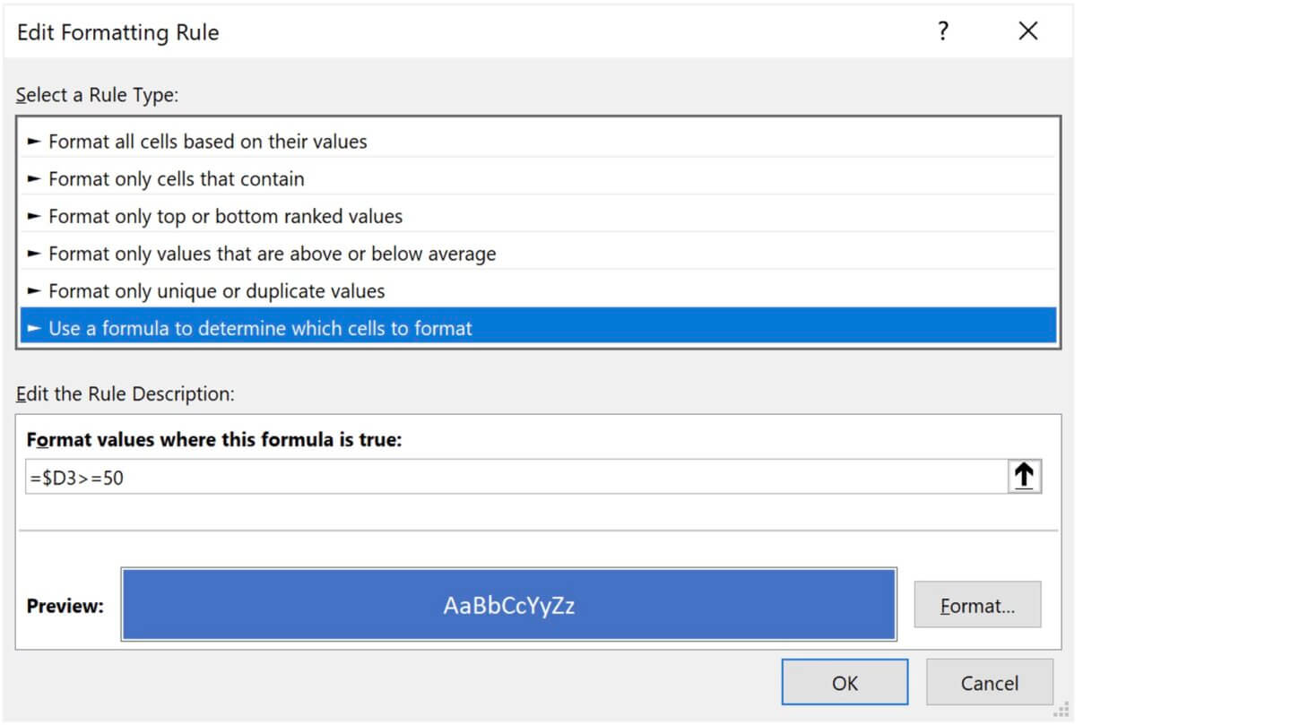
4 Select [ Use a formula to determine which cells to format ] for a rule type.
5 Type the formula [ =$D3>=50 ] for the rule description.
6 Click on the Format button.
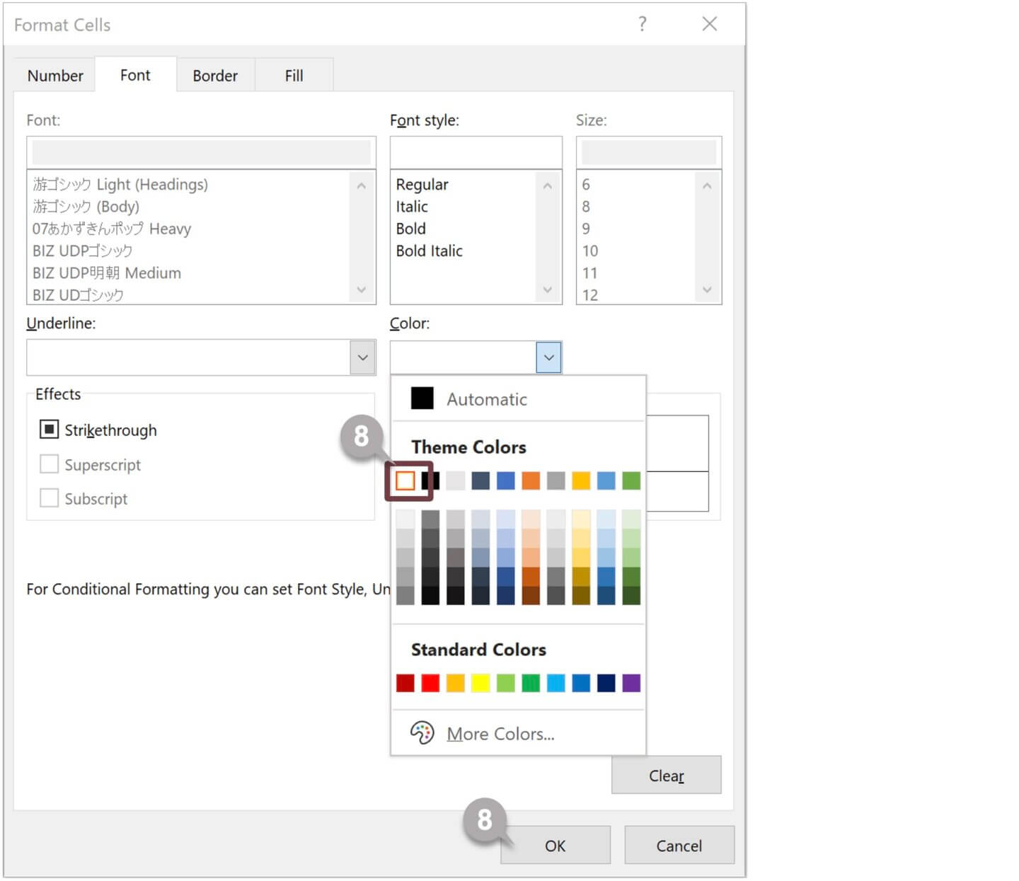
7 The Format Cells dialog box will appear.
8 Click the Fill tab and select a blue color. Click the Font tab, select white color, and click the OK button.
9 Click on the OK button.
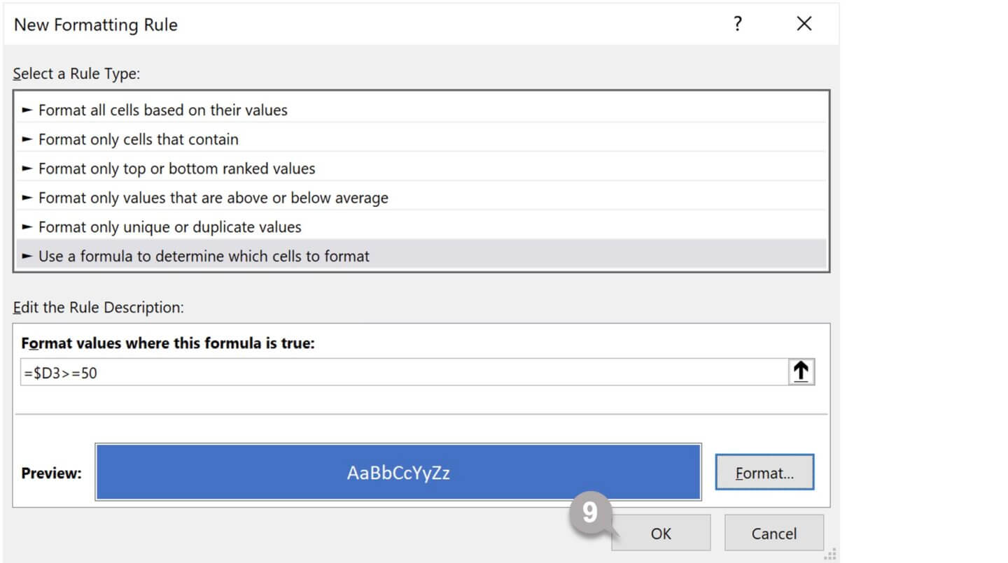
10 The rows for members over 50 years old will be highlighted.
3. How to find the cells with conditional formatting
If you want to edit or clear the rule, you need to know which cells have the setting. Excel has a feature called “Go To” which allows you to find the cells where conditional formatting is set. The steps are below.
1 Select the worksheet that you want to find the setting.
2 In the Editing group on the Home tab, click on Find & Select. Click on Go To from the list.
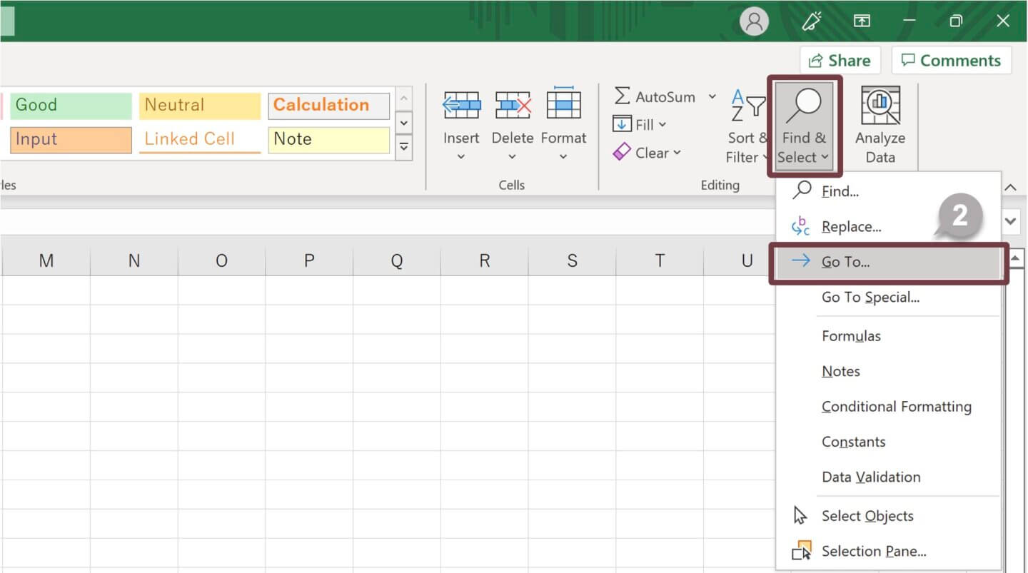
3 The Go To dialog box will appear.
4 Click the Special button.

5 The Go To Special dialog box will appear.
6 Select [ Conditional formats ] and [ All ], and then click the OK button.
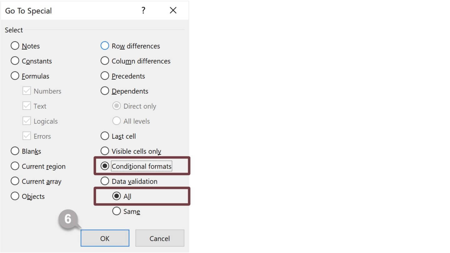
7 All the ranges that have conditional formats in the worksheet will be selected.
–
4. Edit the conditional formatting rule
Follow the steps below to edit the rule for conditional formatting.
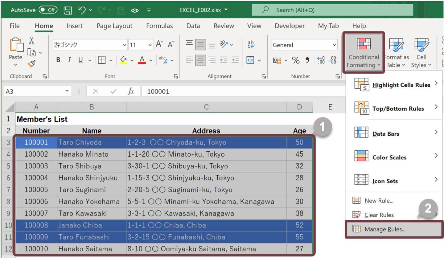
1 Select the ranges that have conditional formats.
2 In the Styles group on the Home tab, click on Conditional Formatting and select Manage Rules from the list.
3 The Conditional Formatting Rules Manager dialog box will appear.
4 Click the Edit Rule button.
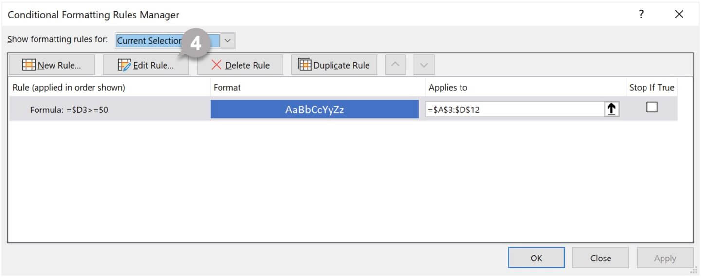
5 The Edit Formatting Rule dialog box will appear.
6 Edit the rule and formats.
TIPS
In the Conditional Formatting Rules Manager dialog box, click the Delete Rule button to clear the rule.
Related Articles

–
