It highlights today’s date in digital calendars such as Outlook Calendar, Google Calendar, etc. Using an Excel feature called Conditional Formatting, you can highlight today’s date just like digital calendars.
This article will show you how to highlight today’s date on three types of monthly calendars using Conditional Formatting.
Language: English Japanese
- 1. Steps to highlighting today’s date
- 2. Formulas to highlight today’s date
- 3. For a calendar with a date entered in one cell
- 4. For a calendar with a date entered in a range of two rows and one column
- 5. For a calendar with a date entered in a range of two rows and two columns
- 6. Copy and paste a calendar that has absolute references on a sheet
–
1. Steps to highlighting today’s date
Let’s highlight the cells of today’s date in monthly calendars in orange and the text in white. The steps are as below.
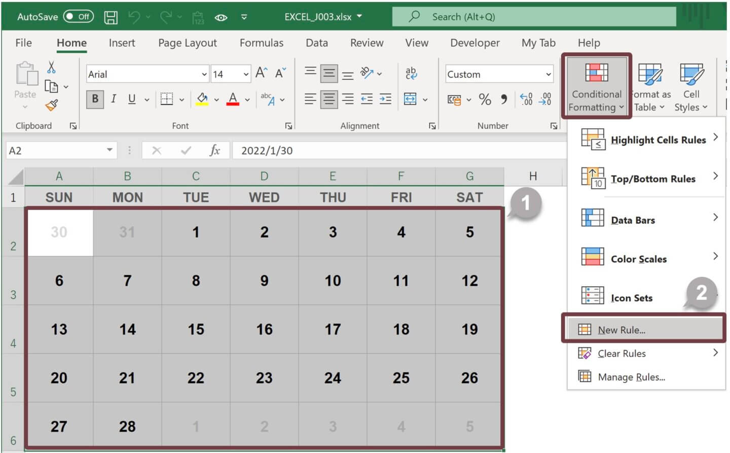
1 Select the range where you want to set the conditional format.
2 In the Styles group on the Home tab, click on Conditional Formatting and select New Rule from the list.
3 The New Formatting Rule dialog box will appear.
4 Select [ Use a formula to determine which cells to format ] for a rule type.
5 Type the formula for the rule description.
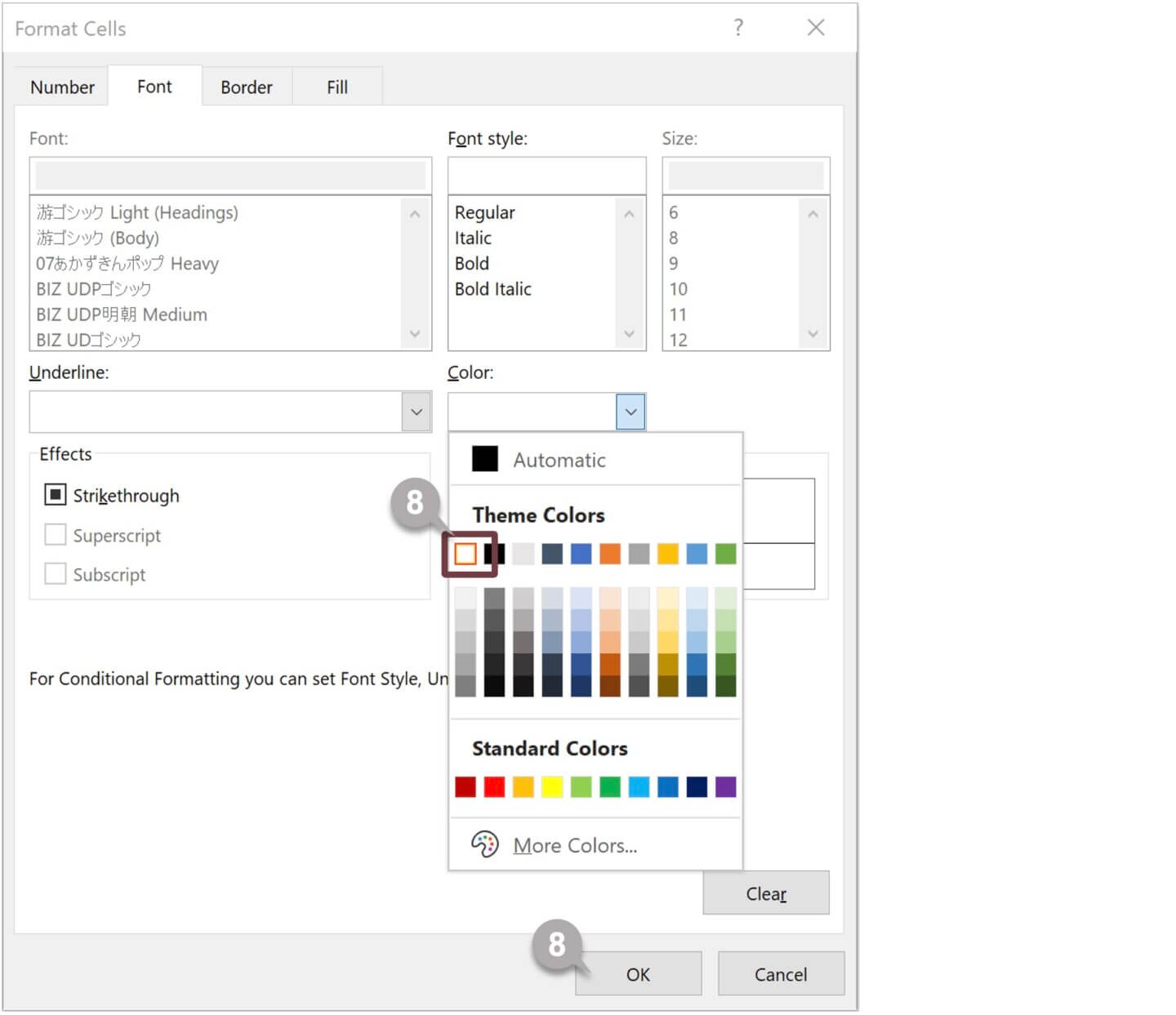
6 Click on the Format button.

7 The Format Cells dialog box will appear.
8 Click the Fill tab and select an orange color. Click the Font tab, select white color, and click the OK button.
9 Click on the OK button on the New Formatting Rule dialog box.
10 The cells of today’s date will be highlighted.
–
2. Formulas to highlight today’s date
To highlight today’s date, use a formula to determine which cells to format. When using formulas, there are relative references and absolute references.
Relative references refer to cells in relation to the location of the cell that contains the formula. When the formula is moved, it references new cells based on their location.
Absolute references always refer to the same cell, even when the formula is copied and pasted. Absolute references are indicated with dollar signs ($) in formulas.
| Absolute column & row reference | $A$1 | The column and row remain constant no matter where the formula is pasted. |
| Absolute column reference | $A1 | The column remains absolute no matter where the formula is pasted, but the row updates relatively. |
| Absolute row reference | A$1 | The row remains absolute no matter where the formula is pasted, but the column updates relatively. |
| Relative column & row reference | A1 | The column and row update where the formula is pasted. |
In this article, I will show you how to highlight today’s date in three types of the monthly calendar. Dates have been input in calendars, and the cells have set formatting to display the day.
–
3. For a calendar with a date entered in one cell
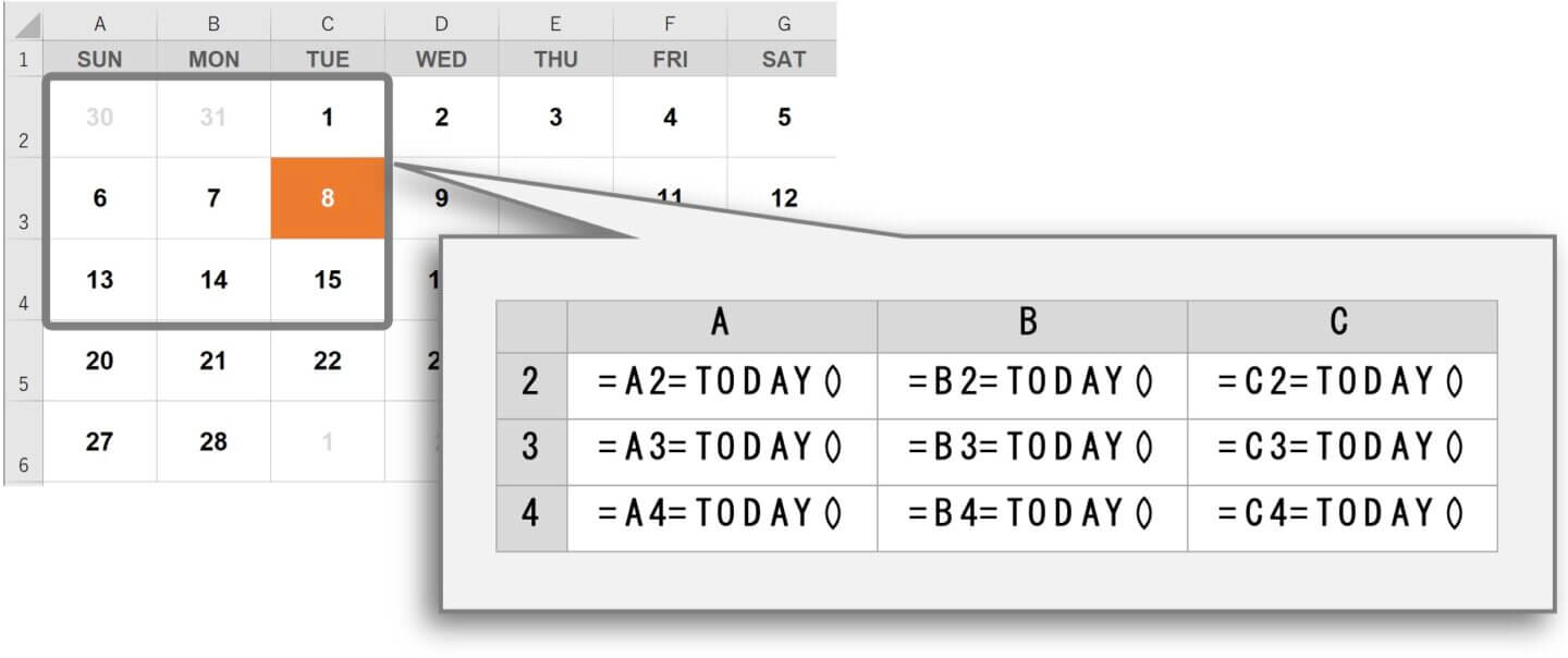
I will show you how to highlight today’s date in the monthly calendar where the date is input in one cell such as the example below.

Follow the instruction [ 1. Steps to highlighting today’s date ] to set formatting. The range for conditional formatting 1 and the formula for the rule 5 are as follows.
| The range for conditional formatting | The formula for the rule |
|---|---|
| Cells A2:G6 | =A2=TODAY() |
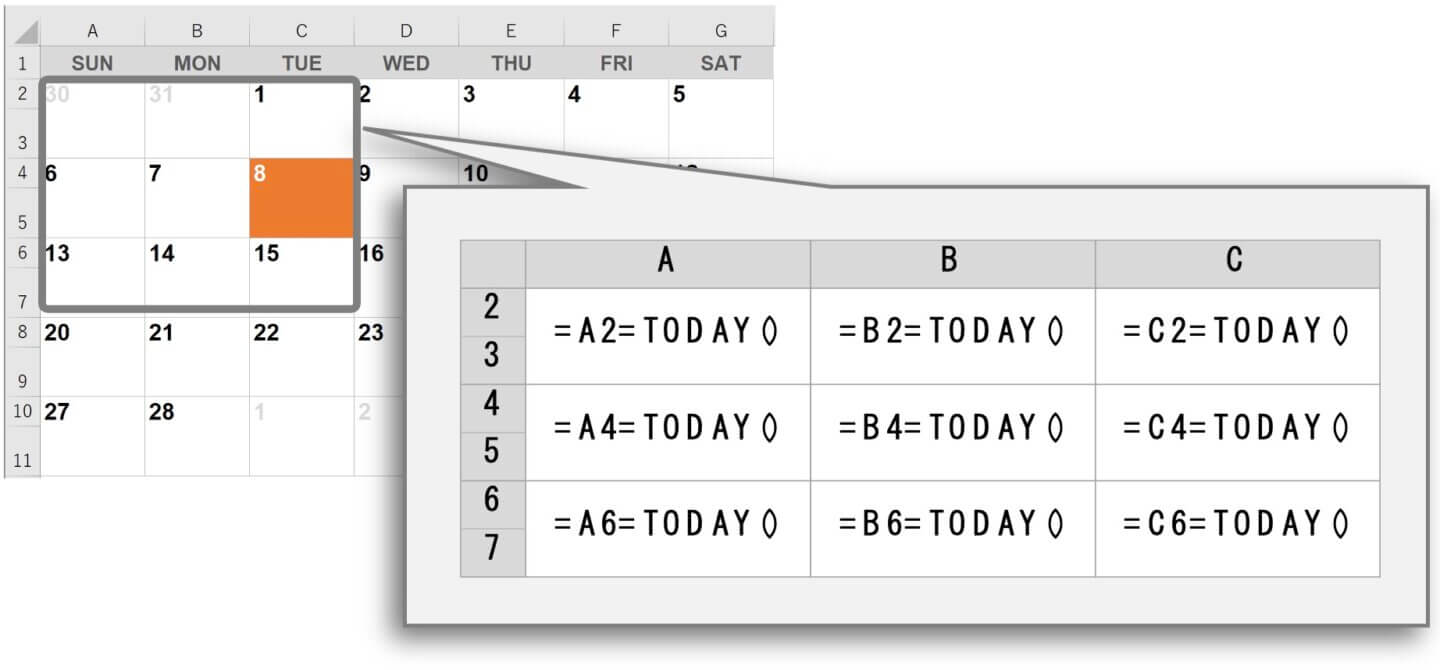
Since the formula entered in the rule is a relative reference, A2 is adjusted, and the following rules are set in cells A2:C4.
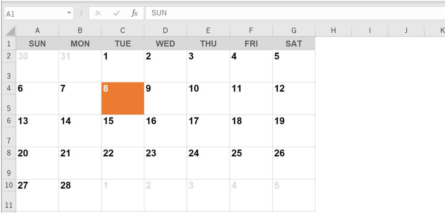
4. For a calendar with a date entered in a range of two rows and one column
In the case of a calendar with a date entered in a range of two rows and one column, follow [ 1. Steps to highlighting today’s date ] for each week and set up five weeks.
The range for conditional formatting 1 and the formula for the rule 5 are as follows.
| Week | The range for conditional formatting | The formula for the rule |
|---|---|---|
| 1st week | Cells A2:G3 | =A$2=TODAY() |
| 2nd week | Cells A4:G5 | =A$4=TODAY() |
| 3rd week | Cells A6:G7 | =A$6=TODAY() |
| 4th week | Cells A8:G9 | =A$8=TODAY() |
| 5th week | Cells A10:G11 | =A$10=TODAY() |
The rule in cell A3 will not be [ A3=TODAY() ] because of the absolute row reference. Since the second row remains absolute, the rule in cell A3 is [ A2=TODAY() ]. The rule in cell B2 is [ B2= TODAY() ] because the column updates relatively. The following rules are set in cells A2:C7.
5. For a calendar with a date entered in a range of two rows and two columns
In the case of a calendar with a date entered in a range of two rows and two columns, follow [ 1. Steps to highlighting today’s date ] for each day and set up days for a month. For the following calendar, you will set up 35 days.

The range for conditional formatting 1 and the formula for the rule 5 are as follows.
| Day | The range for conditional formatting | The formula for the rule |
|---|---|---|
| 1/30 | Cells A2:B3 | =$A$2=TODAY() |
| 1/31 | Cells C2:D3 | =$C$2=TODAY() |
| 2/1 | Cells E2:F3 | =$E$2=TODAY() |
| 2/2 | Cells G2:H3 | =$G$2=TODAY() |
| 2/3 | Cells I2:J3 | =$I$2=TODAY() |
| 2/4 | Cells K2:L3 | =$K$2=TODAY() |
| 2/5 | Cells M2:N3 | =$M$2=TODAY() |
| … | … | … |
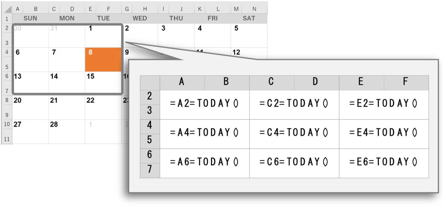
Since absolute column and row reference, column A and row 2 remain constant and the rule for cells A3, B2, and B3 are [ A2=TODAY() ]. The following rules are set in cells A2:F7.
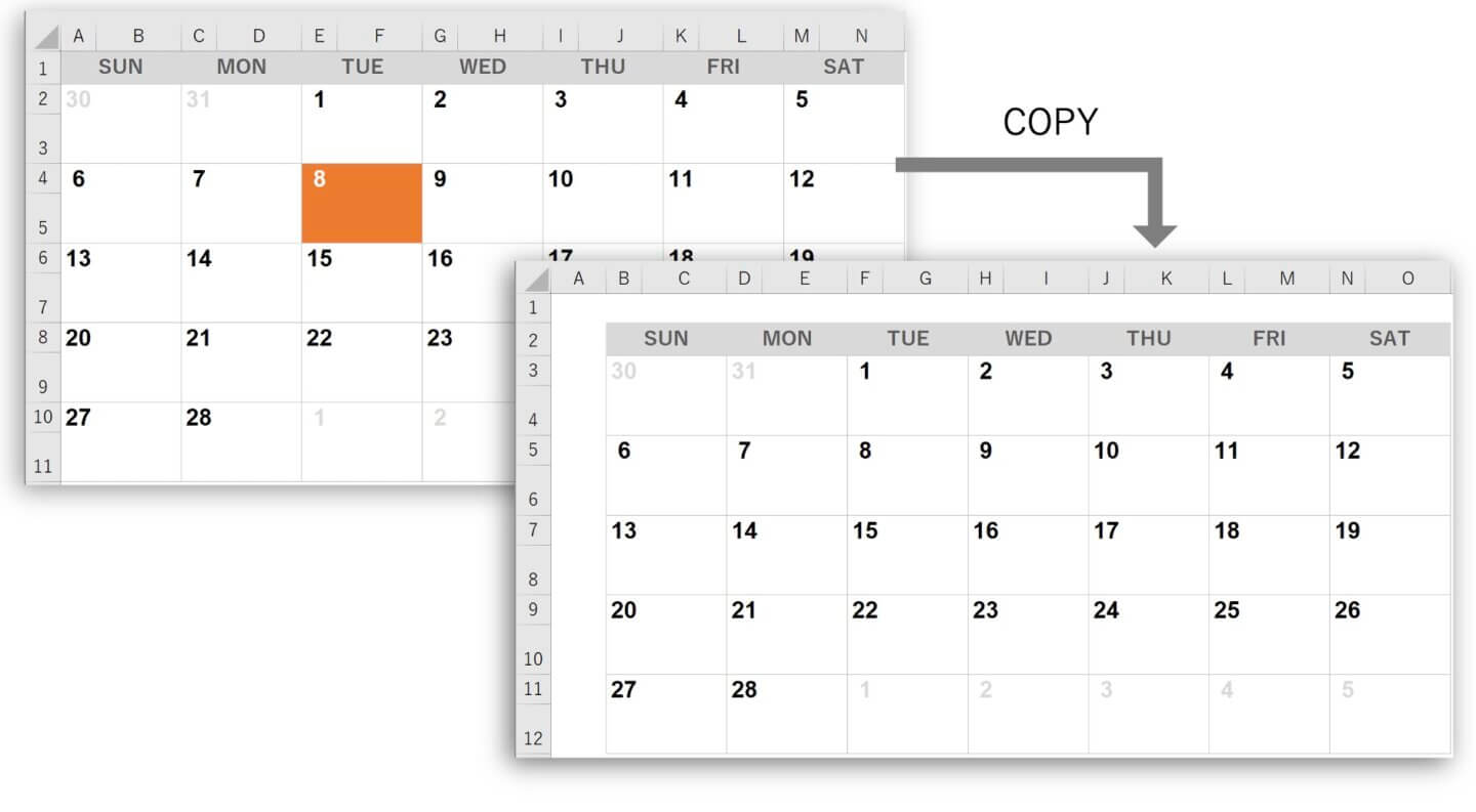
6. Copy and paste a calendar that has absolute references on a sheet
If you copy a calendar that has absolute references and pastes it in a different position or on a different sheet, the date highlighting will not work properly. For example, if you copy cells A1:N11 and paste it into cell B2 on another sheet, the formula for the rule in cells B3:C4 on the pasted sheet are [ =$A$2=TODAY() ], which means it refers to the value in cell A2.
Related Articles

–
